CLCplus Backbone 2023 - Algorith Theoretical Basis Document
Copernicus Land Monitoring Service
Algorithm Theoretical Basis, Land cover classification, Sentinel-2 data, Time series analysis, Temporal Convolutional Neural Network, Deep learning, Bilateral filtering, Interannual calibration, Remote sensing, Geospatial analysis
Contact:
European Environment Agency (EEA)
Kongens Nytorv 6
1050 Copenhagen K
Denmark
https://land.copernicus.eu/
1 Executive summary
The Copernicus Land Monitoring Service (CLMS) provides geospatial information on land cover and its changes, land use, vegetation state, water cycle and Earth’s surface energy variables to a broad range of users in Europe and across the World in the field of environmental terrestrial applications. It supports applications in a variety of domains such as spatial and urban planning, forest management, water management, agriculture and food security, nature conservation and restoration, rural development, ecosystem accounting and mitigation/adaptation to climate change. CLMS is jointly implemented by the European Environment Agency (EEA) and the European Commission DG Joint Research Centre (JRC) and has been operational since 2012.
CLCplus Backbone constitutes the first component of CLMS’ CLCplus Product Suite, which represents a true paradigm change in European land cover/land use monitoring, building on the rich legacy of the European CORINE Land Cover (CLC) flagship product. The CLCplus Backbone is a large scale, seamless and high-resolution inventory of European land cover. It covers the whole of EEA38 territory, the United Kingdom (UK) and the French Overseas Departments (DOMs). The CLCplus Backbone products are freely available, enabling the use by a broad audience, for a wide range of applications.
The CLCplus Backbone 2023 is a geospatial raster product containing 11 basic land cover classes and is based on a time series of high-resolution Sentinel-2 satellite imagery. The input timeseries for this 2023 production covers the reference year ± three months, i.e. 01.10.2022 to 31.03.2024, which is needed to enable the distinction of the 11 land cover classes. CLCplus Backbone maps the dominant (spatially and temporally throughout the specific reference year) land cover for each 10m-raster cell (pixel), applying specific rules according to a comprehensive decision tree. The product has first been produced for the reference year 2018, has been updated for 2021 (excluding the UK) and now as well for 2023, switching to a biennial update cycle and re-including the UK.
This document constitutes the Algorithm Theoretical Basis Document (ATBD), providing a description of the product characteristics, as well as the production methodologies and workflows of the CLCplus Backbone 2023 and the additional quality products.
2 Background of the document
2.1 Scope and objectives
This Algorithm Theoretical Basis Document (ATBD) provides a description of the product characteristics, production methodologies and workflows of the CLCplus Backbone 2023 main (RAS) and its auxiliary layers. The intention of this document is to facilitate an advanced understanding of the product (including its strengths and weaknesses), a description of the input data, the production processes, as well as underlying methodologies and algorithms.
2.2 Content and structure
The ATBD is structured along the different layers, starting with the CLCplus Backbone’s main raster (RAS) layer, i.e. the land cover status classification for 2023, in section 3.1. This includes the provision of the detailed technical product specifications and a stepwise description of the production methodology and algorithms. The subsequent sections provide the technical specifications and a description of the production methodology of the auxiliary layers contained by CLCplus Backbone 2023, i.e. the Raster Confidence Layer (section 3.2), the Raster Data Score Layer (section 3.3) and the Raster Post-Processing Layer (section 3.4).
3 Product descriptions and methodologies
This chapter describes the technical specifications, as well as the methodologies and algorithms used during production of CLCplus Backbone 2023. For detailed information on the class description and nomenclature applied with CLCplus Backbone 2023, please have a look at the corresponding Product User Manual [AD-1AD-1]AD-1.
3.1 CLCplus Backbone 2023 raster (RAS)
The CLCplus Backbone 2023 raster layer (RAS) is a 10m pixel-based land cover map, based on Sentinel-2 data for the reference year 2023 (± 3 months). Each pixel shows the dominant land cover among the 11 basic land cover classes.
3.1.1 Technical product specifications
The technical product specifications for the CLCplus Backbone 2023 are presented below, in Table 1.
3.1.2 Production algorithm and methodology
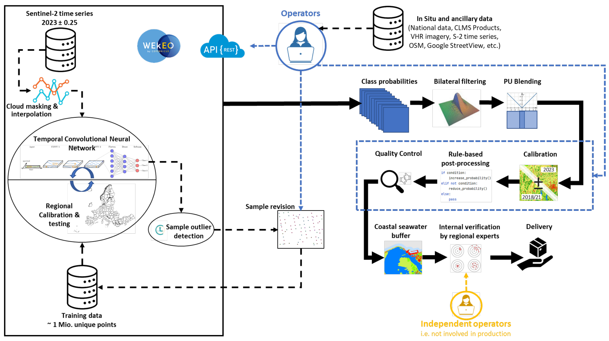
This section provides a methodological description of the production approach for the CLCplus Backbone 2023. Figure 1 shows the general workflow diagram of the production. The most important processing steps are subsequently described in detail.
Technical specifications of the CLCplus Backbone:
Name: CLCplus Backbone Raster
Acronym: RAS
Product family: CLMS_CLCPLUS
Summary: CLCplus Backbone is a spatially detailed, large scale, EO-based land cover inventory. The CLCplus Backbone RASlayer is a 10m pixel-based land cover map based on a Sentinel-2 time series from October 2022 to March 2024 and auxiliary features. For each pixel it shows the dominant land cover among the 11 basic land cover classes.
Reference year: 2023
Geometric resolution: Pixel resolution 10m x 10m, fully conform with the EEA reference grid
Coordinate Reference System: European ETRS89 LAEA projection / WGS84 and the respective UTM zone for the French DOMs
Coverage: 6.002.105 km² (covering the full EEA38 + UK)
Geometric accuracy (positioning scale): Equals Sentinel-2 positional accuracy in 2023 (< 9m at 95.5 % confidence level)
Thematic accuracy: 90 % overall accuracy, not more than 15 % omission errors and 15 % commission errors per class (the amount of omission and commission errors for particular difficult classes such as Low-growing woody plants and Lichens and Moses might regionally exceed those thresholds)
Data type: 8bit unsigned raster with LZW compression
Minimum Mapping Unit (MMU): Pixel-based (no MMU)
Necessary attributes: value, count, Class_name, Area_km2, Area_perc
Raster coding (thematic pixel values):
1: Sealed
2: Woody needle leaved trees
3: Woody broadleaved deciduous trees
4: Woody broadleaved evergreen trees
5: Low-growing woody plants
6: Permanent herbaceous
7: Periodically herbaceous
8: Lichens and mosses
9: Non and sparsely vegetated
10: Water
11: Snow and ice
253: Coastal seawater buffer
254: Outside area
255: No data
Metadata: XML metadata files according to INSPIRE metadata standards
Delivery format: Cloud optimized GeoTIFFs as 100x100km tiles incl. pyramids and embedded colour map (*.tif), attribute table (*.aux.xml), and INSPIRE-compliant metadata in XML format (*.xml)
3.1.3 Input data
The main input data source for the raster classification was Sentinel-2 (S-2) time-series data, covering a period of 1.5 years, i.e. the reference year ±3 months. Since the production of the reference year 2021, the input time series was shortened to the reference year ±3 months compared to the reference year 2018 which was still produced with reference year ±6 months. This change was performed in order to reduce the data volume and processing efforts, and to enable a timelier production of the respective reference years.
Initially, all S-2 scenes at processing level L2A and with a cloud coverage lower than 80% were retrieved from Amazon Web Services (AWS), where the S-2 data is available as Cloud Optimized GeoTIFFs (COGs). If already available at the time of the production start (i.e. beginning of April 2024), Collection-1 data (i.e. ESA S-2 processing baseline ≥ 5.0) was used. If for a certain part of the production AOI and/or time within the reference period, Collection-1 was not available, the time series was complemented with pre-Collection 1 data (i.e. ESA S-2 processing baseline 4.00). This was mainly the case for the period from October to December 2022.
Cloud-masks were computed using the Scene Classification Layer (SCL) provided with each L2A scene by ESA. The S-2 COGs were processed in their native WGS84 UTM projection. After masking out clouds and cloud shadows, all valid observations were taken into account to interpolate an equidistant time-series with a 10-day interval (resulting in a total of 54 timesteps). This processing step included the S-2 bands B1, B3, B4, B5, B8, B9, B11, B12 and four spectral indices, i.e. the Normalized Difference Vegetation Index (NDVI), the Normalized Difference Water Index (NDWI), the Normalized Difference Moisture Index (NDMI) and the Normalized Burn Ratio (NBR). The included 20m S-2 bands were therefore resampled to 10m spatial resolution, applying nearest neighbour resampling. The resulting inputs for the classification were therefore 12 separate raster layers for all features (i.e. 8 S-2 bands and 4 spectral indices), each containing 54 raster bands with the values of the 54 equidistant time steps, described above.
The use of the above bands and indices turned out to provide the best ratio of processing effort and resulting quality. Additional input data to support the classification in particularly difficult areas (i.e. Sentinel-1 time-series, mono-temporal auxiliary features extracted from DEMs, distance features derived from existing LC/LU maps) were extensively tested at several test sites during the ramp up phase of the CLCplus Backbone 2018 production. Nevertheless, these tests demonstrated, that the inclusion of such additional features did in most cases not lead to any significant accuracy gains. Considering the overhead in terms of implementation, I/O and computational footprints, such additional data sources were finally not integrated in the workflow for the CLCplus Backbone production. Additional sampling and post-processing strategies were found more efficient, to address remaining issues in the classification results in difficult regions1.
The training and test data required for the model calibration was based on the sample data base (Sample DB) from the 2018 production, which was compiled from various sources, i.e. from adjusted and filtered LUCAS 2018 data, from stratified automated land cover class annotations based on existing CLMS land cover products, as well as from additional visual sample point photo-interpretation that was supported by VHR imagery, NDVI time series and other auxiliary datasets. The latter comprise available national LC datasets, aerial imagery and LiDAR data that were all collected by a European network of involved regional experts back then. The Sample DB has previously been updated for the CLCplus Backbone 2021 reference year production. Another update and revision of the contained training samples was performed for the 2023 reference year (see section b. Model training in chapter 3.1.5) to account for land cover changes since the previous production and to assure the highest possible quality of the training data. In total, the Sample DB comprised more than 1 million sample points.
3.1.4 Production units
The first CLCplus Backbone raster production for the reference year 2018 was stratified into 232 Production Units (PUs) with an average size of approximately 28,000km². The units were delineated targeting homogeneous environmental characteristics based on the Global Environmental Zones (GEnZ version 3) as described by Metzger et al. (2013). The aim of this stratification was to enable a better regional calibration of the model(s) and hence higher accuracies.
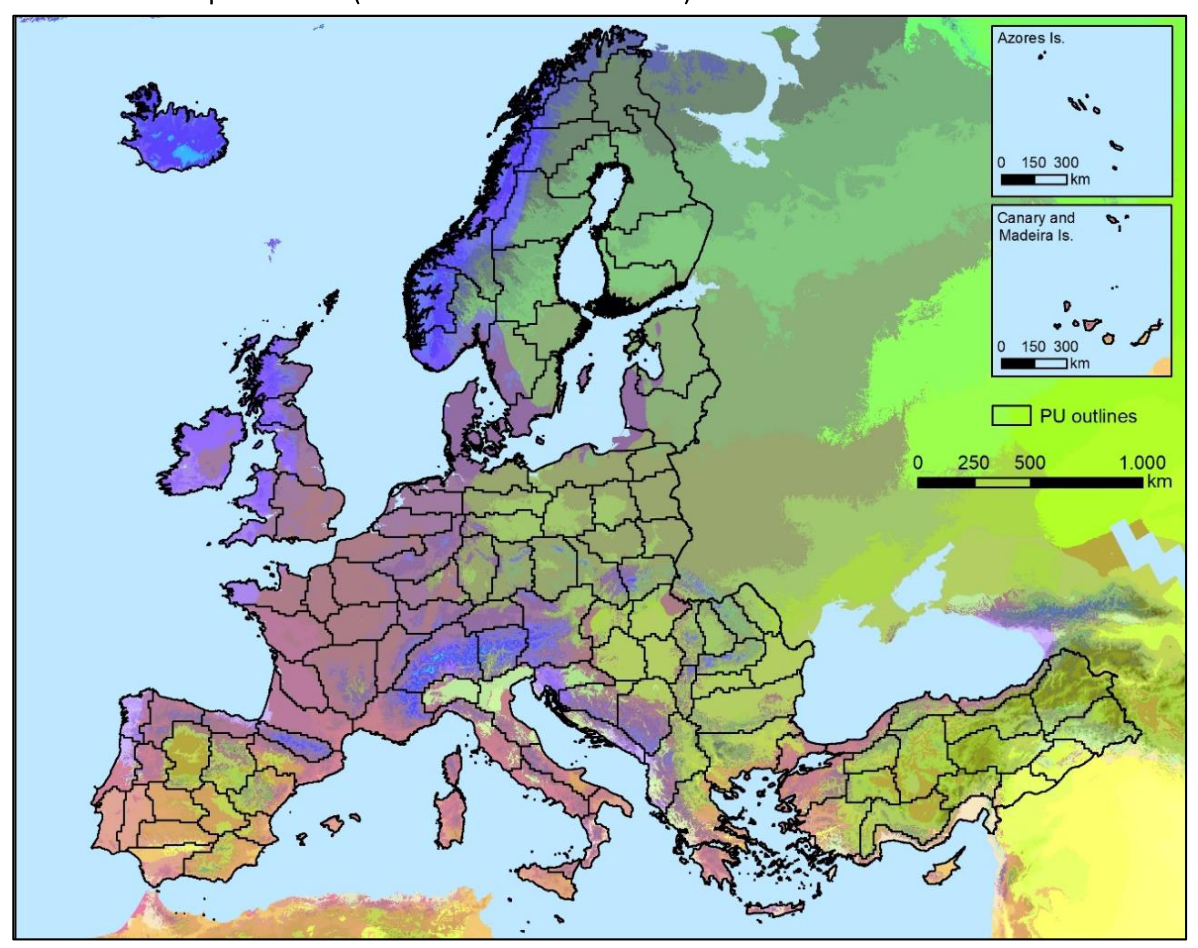
With the CLCplus Backbone 2021 production, the United Kingdom (UK) was excluded and the remaining 223 PUs were aggregated to 132 PUs, as the 2018 production had shown that it would be possible to aggregate some PUs with similar bio-geographical conditions, while retaining good regional calibrations at the same time. As the UK officially re-joined Copernicus in 2024, its territory was added to the ongoing production of the reference year 2023. Accordingly, the PU layout was adapted to now contain 138 PUs that cover the full production area, i.e. the EEA38+UK and the 5 French DOMs. Figure 2 shows the outlines of the PUs for the CLCplus Backbone 2023 production (without the French DOMs).
The homogenous character of the PUs facilitated the regional calibration of the land cover classification models that were trained specifically for each PU. Furthermore, the partitioning allowed to orchestrate and distribute the computation efficiently. The production was generally performed with a spatial overlap of 10 km to neighbouring PU in order to enable post-hoc border harmonization and to avoid any border effects.
3.1.5 Time series classification
The time series classification comprises three main steps, which are described in detail in the following sections:
a. Time series extraction
The S-2 input data time series, as described in section 3.1.3, was in a first step only computed for the training sample locations (i.e. single 10m pixels) and stored per sample point in a dedicated database. This approach enabled an efficient model training as it reduced the data processing effort to a minimum. In a second step, the time series was extracted for the complete Sample DB (see section 3.1.3) of the EEA38+UK area and subsequently used for the separate training of classification models per PU as described below.
b. Model training
The training of classification models was performed in an iterative manner and initially using all training samples from the Sample DB (see section 3.1.3) for a specific PU to train and test models in several stages. The classifier applied was a Temporal Convolutional Neural Network (TempCNN, Pelletier et al. 2019), which proved to be robust, accurate and efficient for operational, large-area analysis of satellite image time series and to outperform well-known classification algorithms such as Random Forest or Recurrent Neural Networks. A cyclic learning rate schedule was used which is known to yield higher accuracies compared to the training, described in the original paper by Pelletier et al. (2019).
The initialmodel training process included an integrated outlier detection using the open-source Python package Cleanlab v2.6.3. (Northcutt et al., 2021) to identify samples where the assigned class label from the previous production deviated from the expected (i.e. modelled) characteristics for the class. This outlier detection was implemented in 15 iterations, where the train and test set compositions changed for each iteration. All samples flagged as potentially conflicting in each of the 15 iterations were finally extracted. The potentially erroneous samples were then reviewed by thematic experts and the class code was updated where land cover change has occurred since the previous production (or in case the sample had been mislabelled in the previous production). Subsequently, the model was trained and tested again with the updated sample data base. In this iteration, 20% of the samples were withheld from training to facilitate model testing and the retrieval of accuracy statistics. Where necessary, the process of sample revisions was repeated until the accuracy metrics achieved with the test set indicated that the product target accuracies were reached.
As a final step, the PU-specific models were trained using all available training samples for the model training, i.e. without splitting the samples into train and test sets. This ensured that the final models were trained on the best-available sample base.
c. Roll out
The trained models were then used to roll out the raster classification to the whole PUs. To this end, the time series data had to be computed with full coverage. The spatial units for this computation were tiles of 25 x 25km (instead of full S-2 scenes) to increase computational performance. The tile grid was nested in the S-2 tile grid to ensure positional accuracy and compliance of all data.
In a second step, the classification was performed on the trained model and input data time series. The classification output was a probability raster with eleven bands - each band representing the per-pixel probabilities for each of the eleven classes. This interim result was then input to the post-processing, as described in the following section.
3.1.6 Post-processing
The post-processing steps applied to the interim per-pixel class probability raster are described in the following sub-sections.
a. Bilateral filtering
A bilateral filter was applied to the class probabilities to reduce the salt and pepper noise (i.e. scattered and isolated pixelsthat are wrongly classified as a result of noise contained in the input imagery and the classification algorithm) in the classification while preserving edges. This type of filter was chosen as it is known to provide a good compromise between computational complexity and accuracy improvements (Schindler 2012). A small window size (win_size=4) and low standard deviation (sigma_spatial=0.8; sigma_color=0.25) was used to parametrize the filter in a way that favoured the preservation of small details while still reducing label noise significantly.
b. Blending
The training data used for model calibration of neighbouring PUs was created with some overlap to ensure consistency in the classification of neighbouring PUs. Nevertheless, differences in the model calibration could still lead to undesired edge effects at the borders of PUs. To circumvent this issue, each PU was initially produced with a buffer of 10km to always ensure an overlap of 20 km between neighbouring PUs. Within this overlap, a distance-weighted averaging of the classification probabilities was performed so that probabilities from both models had equal weights at the centre of the overlap area and de-/increasing weights as a function of the distance from the centre of the overlap.
c. Interannual calibration
Finally, the 2023 class probabilities were calibrated with the combined 2018/2021 probabilities to create best-possible consistency of the CLCplus BB product time series, while allowing for changes in the class assignment where real land cover change or previous misclassifications were detected. For each pixel, the combined probabilities considered the values of the 2018 probabilities where the CLCplus Backbone class remained the same in 2018 and 2021 as well as the values of the 2021 probabilities where it had changed from 2018 to 2021.
As such, the interannual calibration built around the computation of a pixel-based measure of change between the prediction probabilities of 2018/2021 and 2023. Since the probabilities for each of the 11 possible classes per pixel can be interpreted as a point in an 11-dimensional space, the measure of change between two such points, i.e. the probabilities of 2018/2021 (p1821) and 2023 (p2023), can be defined as the Euclidean distance between them:
\[ M_{\text{change}} = \sqrt[2]{ \sum_{i=1}^{11} (p_{2023}^i - p_{1821}^i)^2 } \]
The highest possible value for \(M_{change}\) is given by a change between two class predictions made with 100% certainty, as shown for a change from class 1 to class 2 here:
\[ P_{2023}=(1\ 0\ 0\ 0\ 0\ 0\ 0\ 0\ 0\ 0\ 0) \]
\[ p_{1821}=(0\ 1\ 0\ 0\ 0\ 0\ 0\ 0\ 0\ 0\ 0) \]
\[ M^{max}_{meas}=\sqrt[2]{2}=1.414... \]
With the direction of change known from the comparison of the 2021 and 2023 prediction rasters, it further allowed the implementation of class-specific change thresholds (based on percentiles) and a categorization of pixels in the 2023 raster into low- and high-probability changes. For the majority of pixels experiencing changes between productions, a standard threshold (i.e. the 90th percentile) was used (in theory, 110 change directions are possible). However, change direction-specific thresholds were also applied for particular situations:
very high thresholds for unreasonable changes,such as changes between tree leaf types (i.e. class 2 vs. class 3/4), and
lower thresholds between classes that are more reasonable and likely to change, such as vegetated classes (especially classes 2-7) to Non-sparsely vegetated (class 9) and Sealed (class 1) due to land conversion and/or construction activity).
Based on the above thresholds, changes in the assigned CLCplus Backbone class between 2021 and 2023 were allowed or suppressed, respectively.
d. Further optional post-processing
In cases where significant remaining misclassifications in the raster classification were detected after the cross-calibration during the quality control, those were addressed with a semiautomatic post-processing approach that defined the AOIs of misclassification and subsequently corrected them using available external third-party datasets that had been translated to the CLCplus Backbone nomenclature. This included the correction of omission and commission of sealed surfaces based on the latest release (at the end of the reference period) of Open Street Map (Geofabrik, 2024) and corrections for confusions between classes 6, 7 and partially 5, leveraging data from the Land Parcel Information System (LPIS; where accessible for an affected area). Further, where no adequate auxiliary data was available, a recoding was alternatively based on the expertise of experienced interpreters, who identified the correct class and defined the AOI where changes should be applied. All pixels adapted during this semiautomatic post-processing are documented in the Raster Post-Processing Layer (see section 3.4).
e. Coastal seawater buffer recoding
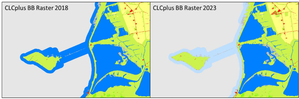
As a last step of the post-processing, the separation of the coastal seawater buffer area from inland water, as introduced in the 2021 production, was performed to enable the derivation of reliable inland water statistics also for countries with significant coastlines. This was done by using the CLMS EU-Hydro coastline product (EEA, 2020) with further manually implemented improvements and the Copernicus EEA39 Boundary Layer with 250 m buffer (EEA, 2019) to derive a mask, covering the respective seawater areas. The underlying pixels were then recoded to a unique raster code with the help of this masking layer. The naming and coding for this technical class is ‘coastal seawater buffer’ with raster code 253, respectively. The raster code 253 is in the range of the outside area and the no data values (254 & 255), which separates it from the 11 thematic land cover classes and does not imply a newly introduced thematic class. Figure 3 shows the CLCplus Backbone 2018 product in comparison to the respective2023 product with the subsequently introduced recoding of the coastal seawater buffer.
3.1.7 Strengths and limitations of the applied methodology
The strongest point of the applied methodology is a generally high accuracy and robustness for the majority of land cover classes and biogeographical regions. This is the result of several elements including:
- The ingestion of a full time series of 1.5 years (i.e. 2023 ± 0.25 years) of Sentinel-2 data, which comprises very rich information on the spectral-temporal dynamics of different land cover classes. This generally enables a very good separability of the 11 target classes and partially even compensates for known shortcomings in the Sentinel-2 L2A input data, such as topographic over-normalization2 on north-to west-facing slopes.
The usage of a state-of-the-art Deep Learning architecture that enables to fully leverage the full time-series without the need for feature engineering orselection which typically leads to a certain loss of information.
A rich sample database of more than 1 million sample points, which have been allocated, curated and quality-checked based on various sources.
A regional calibration approach, which allows to address regional differences and particularly difficult cases in the classification.
A tailored post-processing that comprises the reduction of label noise (i.e. bilateral filtering), assurance of wall-to-wall consistency (i.e. blending) and consistency of the CLCplus Backbone raster time series (i.e. cross-calibration), as well as rule-based reduction of omission and commission errors.
Despite the excellent quality achieved with the applied methodology, some limitations remain. It is worth mentioning, that areas of heterogeneous land cover and small landscape features typically cause an uncertainty due to mixed spectral and temporal signals. Particularly, the classes Low-growing woody plants (class 5) and Lichens and mosses (class 8) have some inherent uncertainty due to i) some fuzziness in the class definition, ii) limited spectral-temporal separability and/or iii) limited reference data, in particular in remote areas. All three factors mentioned above can only be resolved to a certain extent, considering the largely automated approach and the requirements for the timely availability of the product. To a lesser degree, this also concerns areas with intensively managed grassland, where the non-/exposure of bare soil within the reference year cannot always be determined from the input time series with last certainty. As such, confusions of permanent and periodically herbaceous areas (classes 6 vs. 7) may occur.
3.2 Raster Confidence Layer (RASCL)
The Raster Confidence Layer (RASCL) provides information on the confidence of the classifier in the class assignment of each 10m pixel.
3.2.1 Technical product specifications
Below summarizes the technical specifications of the Raster Confidence Layer.
Technical specifications of the Raster Confidence Layer:
Name: CLCplus Backbone Raster Confidence Layer
Acronym: RASCL
Product family: CLMS_CLCplus
Summary: The RASCL is a 10m pixel-based auxiliary layer for the CLCplus Backbone RAS. It provides information about the reliability of the land cover class assignment per pixel.
Reference year: 2023
Geometric resolution: Pixel resolution 10m x 10m, fully conform with the EEA reference grid
Coordinate Reference System: European ETRS89 LAEA projection / WGS84 and the respective UTM zone for the French DOMs
Coverage: 6.002.105 km² (covering the full EEA38 + UK)
Geometric accuracy (positioning scale): equals the Sentinel-2 positional accuracy in 2023 (<9m at 95.5% confidence)
Data type: 8bit unsigned raster with LZW compression
Minimum Mapping Unit (MMU): Pixel-based (no MMU)
Attributes: Value, Count, Confidence
Raster coding:
0-100: Confidence values
254: Outside area
Metadata: XML metadata files according to INSPIRE metadata standards
Delivery format: Cloud optimized GeoTIFFs as 100x100km tiles incl. pyramids and embedded colour map (*.tif), attribute table (*.aux.xml), and INSPIRE-compliant metadata in XML format (*.xml)
3.2.2 Production algorithm and methodology
The RASCL value was calculated for each pixel as the difference between the highest class probability (i.e. the probability of the class that was assigned to the pixel) minus the second highest class probability. This so called (confidence-) margin is conceptually simple, robust and well adapted for multi-class classification problems with variable number of classes. The higher the confidence value, the more reliable the class assignment for a pixel, and vice versa. The value range of RASCL is 0-100.
3.3 Raster Data Score Layer (RASDL)
The Data Score Layer (RASDL) quantifies the number of valid observations in the S-2 image time series which were the input for the equidistant time series interpolation to 10-day intervals.
3.3.1 Technical product specifications
The general technical specifications of the RASDL are provided below.
Technical specifications of the Raster Data Score Layer
Name: CLCplus Backbone Raster Data Score Layer
Acronym: RASDL
Product family: CLMS_CLCplus
Summary: The RASDL is a 10m pixel-based auxiliary layer for the CLCplus Backbone RAS. It is based on a filtered Sentinel-2time series from October 2022 to March 2024 and auxiliary features.
Reference year: 2023
Geometric resolution: Pixel resolution 10m x 10m, fully conform with the EEA reference grid
Coordinate Reference System: European ETRS89 LAEA projection / WGS84 and the respective UTM zone for the French DOMs
Coverage: 6.002.105 km² (covering the full EEA38 + UK)
Geometric accuracy (positioning scale): equals the Sentinel-2 positional accuracy in 2023 (<9m at 95.5% confidence)
Data type: 16bit unsigned raster with LZW compression
Minimum Mapping Unit (MMU): Pixel-based (no MMU)
Necessary attributes: Value, Count, Obs_count
Raster coding:
0-200: Valid observations count
65535: Outside area
Metadata: XML metadata files according to INSPIRE metadata standards
Delivery format: Cloud optimized GeoTIFFs as 100x100km tiles incl. pyramids and embedded colour map (*.tif), attribute table (*.aux.xml), and INSPIRE-compliant metadata in XML format (*.xml)
3.3.2 Production algorithm and methodology
As mentioned above, the RASDL quantifies the number of valid observations in the input time series. A valid observation is in the first place defined as a cloud-free and (cloud-) shadow-free pixel in aS-2 acquisition.
As a preselection, only S-2 acquisitions with an overall cloud coverage below 80% (according to S-2 L2A metadata) were considered for the classification to reduce the data volume and avoid the processing of non-usable image data. The selected S-2 images were then masked based on cloud masks, created for each acquisition, based on the Scene Classification Layer (SCL) provided with the S-2 data. The SCL classes, used for masking the data were classes 2 (dark features/shadows), 3 (cloud shadows), 8 (cloud medium probability) and 9 (cloud high probability). The remaining cloud-free and (cloud-) shadow-free pixels are considered a valid observation and were being counted for each 10m pixel for the complete time window of the reference year ±3 months, i.e. 1.5 years. This count is then stored in a dedicated raster layer.
3.4 Raster Post-Processing Layer (RASPL)
The Raster Post-Processing Layer (RASPL) provides information, if a pixel’s class has been adapted during the optional post processing routine (described in section 3.1.6).
3.4.1 Technical product specifications
The technical product specifications of the Raster Post-processing layer are provided below.
Technical specifications of the Raster Post-Processing Layer
Name: CLCplus Backbone Raster Post-Processing Layer
Acronym: RASPL
Product family: CLMS_CLCplus
Summary: The RASPL is a 10m pixel-based auxiliary layer for the CLCplus Backbone RAS. It provides information of pixels that were re-coded during post-processing of the raster classification.
Reference year: 2023
Geometric resolution: Pixel resolution 10m x 10m, fully conform with the EEA reference grid
Coordinate Reference System: European ETRS89 LAEA projection / WGS84 and the respective UTM zone for the French DOMs
Coverage: 6.002.105 km² (covering the full EEA38 + UK)
Geometric accuracy (positioning scale): equals the Sentinel-2 positional accuracy in 2023 (<9m at 95.5% confidence)
Data type: 8bit unsigned raster with LZW compression
Minimum Mapping Unit (MMU): Pixel-based (no MMU)
Raster coding:
0: No change during post-processing
1: Recoded during post-processing
254: Outside area
Attributes: Value, Count, Class_name
Metadata: XML metadata files according to INSPIRE metadata standards
Delivery format: Cloud optimized GeoTIFFs as 100x100km tiles incl. pyramids and embedded colour map (*.tif), attribute table (*.aux.xml), and INSPIRE-compliant metadata in XML format (*.xml)
3.4.2 Production algorithm and methodology
The RASPL provides information, if a pixel’s class code has been adapted during the postprocessing. This excludes potential changes coming from the bilateral filtering and the interannual calibration, being part of the general post-processing, but forming integral processing steps towards the initial class assignment. Only pixels that were changed thereafter, i.e. in the additional optional post-processing steps for further refinement of the initial class assignment, are flagged as ‘Recoded during post-processing’ in the RASPL.
The adapted areas are simply identified by a comparison of the final classification result with the interim outcome after the interannual calibration step. Where the assigned class codes do not match, the pixels are assigned with value 1 and value 0 is assigned to all unchanged pixels.
4 Terms of use and product technical support
4.1 Terms of use
The Terms of Use for the product(s) described in this document acknowledge the following:
Free, full and open access to the products and services of the Copernicus Land Monitoring Service is made on the conditions that:
When distributing or communicating Copernicus Land Monitoring Service products and services (data, software scripts, web services, user and methodological documentation and similar) to the public, users shall inform the public of the source of these products and services and shall acknowledge that the Copernicus Land Monitoring Service products and services were produced “with funding by the European Union”.
Where the Copernicus Land Monitoring Service products and services have been adapted or modified by the user, the user shall clearly state this.
Users shall make sure not to convey the impression to the public that the user’s activities are officially endorsed by the European Union.
The user has all intellectual property rights to the products he/she has created based on the Copernicus Land Monitoring Service products and services.
Consult Data policy — Copernicus Land Monitoring Service for further details.
4.2 Citation
When planning a publication (scientific, commercial, etc.), it shall explicitly mention:
“This publication has been prepared using European Union’s Copernicus Land Monitoring Service information; <insert all relevant DOI links here, if applicable>”
When developing a product or service using the products or services of the Copernicus Land Monitoring Service, it shall explicitly mention:
“Generated using European Union’s Copernicus Land Monitoring Service information;<insert all relevant DOI links here, if applicable>”
When redistributing a part of the Copernicus Land Monitoring Service (product, dataset, documentation, picture, web service, etc.), it shall explicitly mention:
“European Union’s Copernicus Land Monitoring Service information; <insert all relevant DOI links here, if applicable>”
Consult Data policy — Copernicus Land Monitoring Service for further details.
4.3 Product technical support
Product technical support is provided by the product custodian through Copernicus Land Monitoring Service – Service desk. Product technical support does not include software specific user support or general GIS or remote sensing support.
More information on the products can be found on the Copernicus Land Monitoring Service website (https://land.copernicus.eu/)
5 List of abbreviations
| Abbreviation | Name | Reference |
|---|---|---|
| ADs | Applicable Documents | |
| AI | Action Item | |
| AOI | Area Of Interest | |
| ATBD | Algorithm Theoretical Basis Document | |
| BB | (Corine Land Cover plus) Backbone | |
| CLC | CORINE Land Cover | |
| CLCplus | CORINE Land Cover plus | |
| CLMS | Copernicus Land Monitoring Service | https://land.copernicus.eu/en |
| COG | Cloud Optimized GeoTiff | |
| DB | Data Base | |
| DOMs | French Overseas Departments | |
| EEA | European Environment Agency | www.eea.europa.eu |
| EEA38 | The 32 member and 6 cooperating countries of the EEA | https://land.copernicus.eu/en/faq/general-questions/what-is-eea38 |
| EEA39 | The 39 member and cooperating countries of the EEA, before UK´s withdrawal | |
| EO | Earth Observation | |
| ESA | European Space Agency | https://www.esa.int/ |
| FWC | Framework Service Contract | |
| INSPIRE | Infrastructure for Spatial Information in Europe | https://knowledge-base.inspire.ec.europa.eu/index_en |
| JRC | European Commission DG Joint Research Centre | Joint Research Centre |
| LC | Land cover | |
| LiDAR | Light Detection and Ranging | |
| LPIS | Land Parcel Information System | LPIS - land parcel identification system a.k.a. identification system for agricultural parcels -Guidance and Tools for CAP (GTCAP) - EC Public Wiki |
| LU | Land use | |
| LUCAS | Land Use/Cover Area frame Survey | LUCAS - Land use and land cover survey - Statistics Explained |
| L2A | Level 2A (processing level of Sentinel-2 satellite data) | https://sentiwiki.copernicus.eu/web/s2-processing#S2Processing-L2AAlgorithmsS2-Processing-L2A-Algorithmstrue |
| MMU | Minimum Mapping Unit | |
| NBR | Normalized Burn Ratio | |
| NDMI | Normalized Difference Moisture Index | |
| NDVI | Normalized Difference Vegetation Index | |
| NDWI | Normalized Difference Water Index | |
| OSM | Open Street Map | https://www.openstreetmap.org |
| PU | Production Unit | |
| RfS | Request for Service | |
| RAS | CLCplus BB Raster Product | |
| RASCL | Raster Confidence Layer | |
| RASDL | Raster Data Score Layer | |
| RASPL | Raster Post-processing Layer | |
| SC | Specific Contract | |
| SCL | Scene Classification Layer | |
| S-2 | Sentinel-2 | |
| UK | United Kingdom | |
| VHR | Very High Resolution |
6 References
EEA (European Environment Agency) (2019). Copernicus EEA39 Boundary Layer with 250 m buffer (raster 10m), version 3, Jan. 2019. https://sdi.eea.europa.eu/catalogue/srv/api/records/1ba7fc7e-490f-45b2-875c-5ca9742f2c0d [31.01.2025]
EEA (European Environment Agency) (2020). EU-Hydro River Network Database 2006-2012 (vector), Europe - version 1.3, Nov. 2020. https://doi.org/10.2909/393359a7-7ebd-4a52-80ac-1a18d5f3db9c [27.03.2025]
Geofabrik (2024). Open Street Map data, accessed on 2024/04/04. https://www.geofabrik.de/geofabrik/openstreetmap.html [27.03.2025]
Metzger, M. J., Bunce, R. G., Jongman, R. H., Sayre, R., Trabucco, A., & Zomer, R. (2013). A high‐resolution bioclimate map of the world: a unifying framework for global biodiversity research and monitoring. Global Ecology and Biogeography, 22(5), 630-638.
Pelletier, C., Webb G.I. & Petitjean, F. (2019). Temporal Convolutional Neural Network for the Classification of Satellite Image Time Series. Remote Sensing 11, no. 5: 523. https://doi.org/10.3390/rs11050523
Northcutt, C., Jiang, L., & Chuang, I. (2021). Confident learning: Estimating uncertainty in dataset labels. Journal of Artificial Intelligence Research, 70, 1373-1411. https://doi.org/10.48550/arXiv.1911.00068 [27.03.2025]
Schindler, K. (2012). An overview and comparison of smooth labeling methods for landcover classification. IEEE Transactions on Geoscience and Remote Sensing, 50(11), 4534-4545. https://ieeexplore.ieee.org/document/6198886 [27.03.2025]
7 Document history
| Version | Date | Short description of changes |
|---|---|---|
| 1.2 | 01.04.2025 | Initial published version |
8 Applicable documents
| ID | Applicable document |
|---|---|
| AD-1 | CLCplus Backbone 2023 - Product User Manual (PUM) |
9 Change Log
| Date | Version | Summary |
|---|---|---|
| 2025-12-02 | 1.2.0 | Initial release |
Footnotes
The difficulties in those areas are manifold and range e.g. from very dry conditions, causing low vegetation cover and soil signal contamination in the Mediterranean, to illumination effects/shadows and short vegetation cycles (prolonged snow cover) in the northern areas of Europe.↩︎
This issue has been described in S2 MPC - Level-2A Algorithm Theoretical Basis Document (Ref. S2-PDGS-MPC-ATBDL2A; https://step.esa.int/thirdparties/sen2cor/2.10.0/docs/S2-PDGS-MPC-L2A-ATBD-V2.10.0.pdf)↩︎