European Ground Motion Service (EGMS) - Product Description and Format Specification

Copernicus Land Monitoring Service

This document provides a comprehensive description of the European Ground Motion Service (EGMS) products, which are part of the Copernicus Land Monitoring Service. It details the specifications, formats, attribute tables, and metadata associated with the EGMS Basic, Calibrated, and Ortho products. Furthermore, the document outlines the processing methodologies employed, including InSAR techniques and the integration of GNSS data for georeferencing, ensuring users have a thorough understanding of the products and their appropriate use.

Published

January 10, 2025

Keywords

InSAR displacement data, Satellite line-of-sight, GNSS time-series data, Earth centred reference frame, Vertical and east-west displacements, 100 m gridded data, ETRS89-LAEA projection, Temporal coherence, Amplitude Dispersion Index, A-EPND reference model

European Environment Agency (EEA)
Kongens Nytorv 6
1050 Copenhagen K
Denmark
https://land.copernicus.eu/

1 Introduction

1.1 Scope

To enable full use of the European Ground Motion Service (EGMS), it is necessary to have an understanding of its products. This document provides a full description of EGMS products, along with details of specifications, formats, attribute tables and metadata, plus other information considered of use to users of the service.

After referring to related documents, this section continues with some InSAR-specific definitions to aid understanding of the service specifications. Section 3 then goes on to discuss product map projections, followed by sections detailing product specifications, attributes and formats. Section 7 discusses user downloading before the document ends with detail of ancillary datasets used in EGMS production.

2 EGMS Product Overview

The European Ground Motion Service provides three main InSAR products for visualisation, analysis and download by users of the service’s dissemination platform.

The EGMS Basic product
The EGMS Calibrated product
The EGMS Ortho product

An outline of each follow:

2.1 The EGMS Basic product

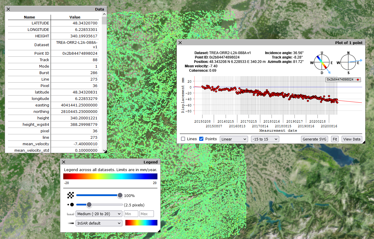
Figure 1 EGMS Basic (L2a) product. Provided as a 2D, colour-coded by average velocity, map. Displacement data provided in the satellite line-of-sight, and in radar geometry, with annotated geolocalisation and quality measures per measurement point. A time series plot is associated with each point.

The EGMS Basic product provides InSAR displacement data provided in the satellite line-of-sight, with annotated geolocalisation and quality measures per measurement point (MP). Satellite line-of-sight means that measurements are projected along the imaginary line which connects the satellite to the target, and which have to be reprojected to assume the meaning of vertical/horizontal displacement.

The product is provided as a 2D map of InSAR measurement points, colour-coded by average velocity. A time series plot is associated with each point.

Significantly, Basic products are spatially referenced to a virtual reference point, whose time series is derived by a statistical analysis of the dataset. As a consequence, the provided measurements are meaningful just considering the processed area. It is not possible to compare deformations from adjacent areas belonging to different products of the same level. The time series are temporally referenced to the value of the deformation model at time T₀=0. Please refer to [RD1] for a description of the selected approaches’ rationale.

Production of the EGMS Basic product is a necessary first step and input to the more advanced EGMS Calibrated product. EGMS Basic products are provided as two discrete datasets; one made from the SAR data acquired orthogonal to the satellite ascending trajectory (south to north), the other from data acquired orthogonal to the descending trajectory (north to south). Please refer to documents [RD1] and [RD2] for additional details on ascending and descending acquisitions.

2.2 The EGMS Calibrated product

The EGMS Calibrated product is considered the main EGMS product as it serves the needs of most users. It is fundamentally the same as the Basic product but enhanced by the InSAR MP displacement values being referenced to model derived from GNSS time-series data, thereby making the InSAR measurements absolute (with reference to an Earth centred reference frame). Calibrated products, containing absolute measurements, overcome the intrinsic limits of the Basic ones, being possible to compare deformations from adjacent areas belonging to different products of the same level.

As with Basic products, the Calibrated product is provided as two discrete datasets, one in ascending geometry, the other in descending geometry.

Some isolated islands may not have GNSS data available. For these areas, Calibrated products are produced by harmonizing Basic products with respect to each other, and then adjusting the mean ground velocity to zero. Measurements of any displacements on such islands are not referenced against the GNSS-derived datum, but a local InSAR MP.

2.3 The EGMS Ortho product

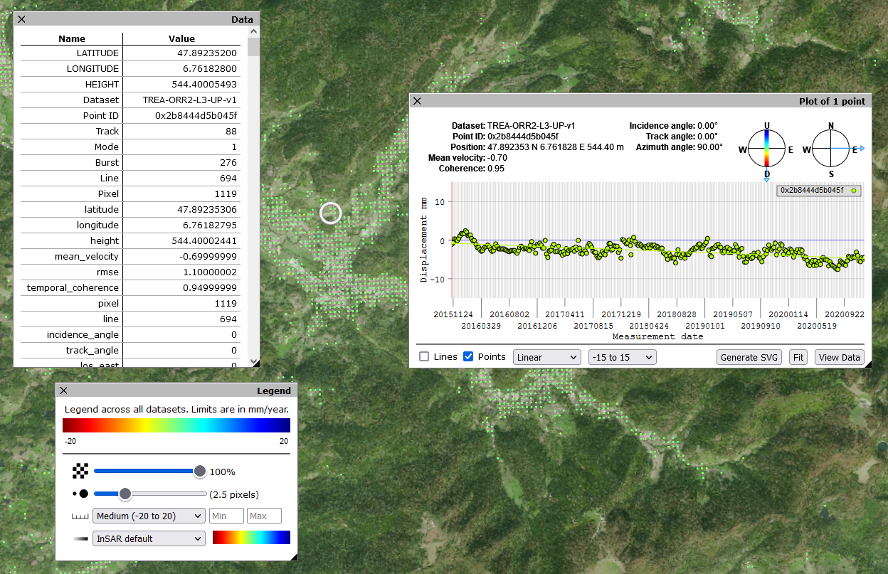
Figure 2 EGMS Ortho product. Absolute, vertical displacement. The gridded nature of the data is clearly visible.

The EGMS Ortho product exploits the discrete look-angles provided by the Calibrated product to derive two further layers; one of purely vertical displacements, the other of purely east-west displacements. Both layers are resampled to a 100 m grid to coincide with other Copernicus products. Vertical and east-west displacement components can be estimated taking advantage of the prior information coming from GNSS data. Refer to RD1 for more details about the Ortho products generation process.

The main benefit of Ortho products is ease of understanding to those new to InSAR as the data-acquisition geometry need not be considered. However, such decomposed data can still prove valuable even to InSAR experts when considering phenomena that might include non-vertical displacements such as those relating to tectonics or landslides.

In the following, some characteristics of the EGMS Ortho product:

Coverage: To make the Ortho product, both ascending and descending geometry Calibrated products are needed. In some areas of high topographic relief, the usual geometric artefacts associated with radar remote sensing (layover, foreshortening and shadow) prevent 100% coverage. In such areas, there are no EGMS Ortho measurements.
Not full-3D: Each Sentinel-1 satellite is near-polar-orbiting with a side-looking radar. The ‘range-finding’ echoes of the SAR instrument consequently become less sensitive as the direction of any ground displacement approaches that of the satellite flightpath, i.e., north-south. Importantly, any ground movements in these directions will not be measured directly by InSAR but reintroduced from the GNSS data (please refer to RD1). In fact, north-south displacement components are not available for any MP, since they are estimated from GNSS data, characterized by a much lower spatial resolution than InSAR measurements. Therefore, vertical, and east-west components are estimated thanks to a spatial interpolation of the information available. This approach, however, does not introduce a significant bias in the measurements, apart from area affected by strong spatial variations of north-south displacements.
Spatial sampling: The ascending and descending Calibrated products that make the Ortho product have different acquisition geometries, meaning that the distribution of MPs is not identical between the two datasets. To ensure that both datasets represent the same area of ground, the data is averaged to a common 100 m grid, this particular spacing chosen to coincide with other Copernicus services and it is a good compromise between resolution and spatial coverage of the database.
Temporal sampling: in general, the temporal sampling of the satellite tracks contributing to the Ortho product is not aligned. This happens because L2b products, from which L3 are derived, exhibit acquisition patterns shifted in times on a track basis. Moreover, there may be holes in the datasets (e.g., missed acquisition, especially in 2015). In order to define a common temporal grid, for the baseline all time-series will start on January 2016 and end on December 2021, with regular six-day temporal sampling with origin on 3-April-2014 (launch date of S1A). A regular sampling will be maintained whenever possible, even if, in correspondence of huge gaps in the L2b products time series used to generate the L3 level, customized solutions may be adopted. Please refer to document RD1 for further details on L3 products generation.

2.4 The EGMS A-EPND GNSS-based reference model

The process of generating the Calibrated (see section 2.2) and the Ortho (see Section 2.3) products requires the availability of a reference model derived from GNSS data. The augmented EPND (A-EPND) model is produced based on GNSS data from various sources, with the EUREF Densification product (EPND) as the main source. In order to exploit the strengths of both InSAR and GNSS data, the reference model contains average velocities in 3D (east, north, up) on a 50-km grid. Deviations from the constant velocity model, as well as motion on shorter spatial scales than the reference model, will be estimated from InSAR data with high spatial density. Further details about the A-EPND model can be found in RD8.

3 Projection and Datum

Basic and Calibrated products are point databases (i.e., ‘vector data’ in GIS jargon). As such, the choice of projection and datum does not affect the product quality - they can be reprojected on-the-fly without any geometric distortion. Modern GIS platforms can make such reprojections rapidly, so the choice of projection for storage and delivery of these products is not critical. However, a uniform projection is used for EGMS products using the European Grid (ETRS89-LAEA), a standard based upon the ETRS89 Lambert Azimuthal Equal-Area projection coordinate reference system, with the centre of the projection at the point 52° N, 10° E. In addition, non-projected (geographic) coordinates using the WGS84 datum are annotated for each measurement point in Basic and Calibrated products.

EGMS Ortho products (which are in raster format) are based upon a 100 m grid, where each cell is dependent on the chosen projection and datum. When such data are reprojected, they must be resampled, and thus are susceptible to geometric distortions.

4 EGMS Product Specifications

This section details the specifications for each of the three EGMS products. Note, for Basic and Calibrated products, the specifications are common to both ascending and descending geometries. This does not apply to Ortho products that are made from the decomposition of both geometries.

4.1 EGMS Basic product specifications

Table 1 EGMS Basic product specifications
ITEM	Specification
Tiling	Original burst segmentation of the reference image.
Reference system	ETRS89-LAEA.
File name convention	Data from each burst are contained in single CSV format file the name of which is in the format EGMS_L2a_xxx_yyyy_IWz_ww_aaaa_bbbb_c.csv (e.g., EGMS_L2a_088_0282_IW2_VV_2018_2022_1.zip), where xxx - Track number yyyy - Progressive index for the burst inside the track z - The swath the burst belongs to ww - Polarization aaaa - First nominal year of the years’ time range in which data are included bbbb - Last nominal year of the years’ time range in which data are included c Version of the delivered data Further details on the file naming convention can be found in section 11.2. Deliverables belonging to the Baseline or to the First update follow the same naming convention with the exception of the suffix _xxxx_yyyy_z, which is not applied.
Format	Vector point.
Header information	For each CSV data file there is a header file in XML format, the name of which is a copy of the name of the relative data file (e.g., EGMS_L2a_xxx_yyyy_IWz_ww_aaaa_bbbb_c.xml). The header file contains metadata useful to identify the origins of each product and to allow reproducibility. The structure of the header file can be found in section 11.1.
Epoch spanned	Baseline - From February 2015 to December 2020 1^st Update - From February 2015 to December 2021 2^nd Update - From January 2018 to December 2022 3^rd Update - From January 2019 to December 2023
Spatial resolution	PS full resolution (single pixel of Sentinel-1 constellation products in Interferometric Wide Swath. Namely, 5 x 20 m), DS better than 100 m.
Temporal resolution	12 days till October 2016 and 6 days from October 2016 onward.
3D geolocation accuracy	Better than 10m.
Mean velocity resolution	Better than 1 mm/year.
Mean velocity STD	0.7 mm/year (1 σ) for MP with coherence greater than 0.7.
Displacement STD	4 mm (1 σ).
MP density	CLC18-1.1.1 ‘Continuous Urban Fabric’: >= 5,000 MP/km². CLC18-1.1.2 ‘Discontinuous Urban Fabric’ and 1.2 ‘Industrial, Commercial, and Transport Units’: >=1,000 MP/km². CLC18-3.3 ‘Open Spaces with Little or no Vegetation’: >=100 MP/km².

4.2 EGMS Calibrated product specifications

Table 2 EGMS Calibrated product specifications
ITEM	Specification
Tiling	Original burst segmentation of the reference image.
Reference system	ETRS89-LAEA.
File name convention	Data from each burst are contained in single CSV format file the name of which is in the format EGMS_L2a_xxx_yyyy_IWz_ww_aaaa_bbbb_c.csv (e.g., EGMS_L2a_088_0282_IW2_VV_2018_2022_1.zip), where xxx - Track number yyyy - Progressive index for the burst inside the track z - The swath the burst belongs to ww - Polarization aaaa - First nominal year of the years’ time range in which data are included bbbb - Last nominal year of the years’ time range in which data are included c Version of the delivered data Further details on the file naming convention can be found in section 11.2. Deliverables belonging to the Baseline or to the First update follow the same naming convention with the exception of the suffix _xxxx_yyyy_z, which is not applied.
Format	Vector point.
Header information	For each CSV data file there is a header file in XML format, the name of which is a copy of the name of the relative data file (e.g., EGMS_L2a_xxx_yyyy_IWz_ww_aaaa_bbbb_c.xml). The header file contains metadata useful to identify the origins of each product and to allow reproducibility. The structure of the header file can be found in section 11.1.
Epoch spanned	Baseline - From February 2015 to December 2020 1^st Update - From February 2015 to December 2021 2^nd Update - From January 2018 to December 2022 3^rd Update - From January 2019 to December 2023
Spatial resolution	PS full resolution (single pixel of Sentinel-1 constellation products in Interferometric Wide Swath. Namely, 5 x 20 m), DS better than 100 m.
Temporal resolution	12 days till October 2016 and 6 days from October 2016 onward.
3D geolocation accuracy	Better than 10 m.
Mean velocity resolution	Better than 1 mm/year.
Mean velocity STD	0.7 mm/year (1 σ) for MP with coherence greater than 0.7.
Displacement STD	8 mm (1 σ).
MP density	CLC18-1.1.1 ‘Continuous Urban Fabric’: >= 5,000 MP/km². CLC18-1.1.2. ‘Discontinuous Urban Fabric’ and 1.2 ‘Industrial, Commercial, and Transport Units’: >=1,000 MP/km². CLC18-3.3- ‘Open Spaces with Little or no Vegetation’: >=100 MP/km².

4.3 EGMS Ortho product specifications

Table 3 EGMS Ortho product specifications
ITEM	Specification
Tiling	100 x 100 km tiles according to EEA recommendations, with south-west corner on a multiple of 100 km in ETRS89-LAEA coordinates (also known in the EPSG Geodetic Parameter Dataset* under the identifier: EPSG:3035. The geodetic datum is the European Terrestrial Reference System 1989 (EPSG:6258). The Lambert Azimuthal Equal Area (LAEA) projection is centred at 10°E, 52°N. Coordinates based on a false easting of 4,321,000 m, and a false northing of 3,210,000 m).
Reference system	ETRS89-LAEA.
File name convention	Two Geo TIFF files for each tile, one for vertical velocity component, and one for east-west. File names are in the format EGMS_L3_EXXNYY_100km_C_aaaa_bbbb_c.tif (e.g., EGMS_L3_E40N28_100km_U_2018_2022_1.tif and EGMS_L3_E40N28_100km_E_2018_2022_1.tif), where XX - Easting coordinate of the South-West corner of the lower left pixel of the tile YY - Northing coordinate of the South-West corner of the lower left pixel of the tile C - Mean velocity component (U for vertical displacement and E for horizontal displacement in the East-West direction) aaaa - First nominal year of the years’ time range in which data are included bbbb - Last nominal year of the years’ time range in which data are included c Version of the delivered data Associated with each tile are also two CSV files, containing the time-series and other parameters for the two mean velocity components. The file names follow the same convention as mean velocity Geo TIFF, except for the file extension (e.g., EGMS_L3_E40N28_100km_U_2018_2022_1.csv and EGMS_L3_E40N28_100km_E_2018_2022_1.csv). The coordinates contained in the vector csv format refer to the centre of the resolution cell. Further details on the file naming convention can be found in section 11.2. Deliverables belonging to the Baseline or to the First update follow the same naming convention with the exception of the suffix _xxxx_yyyy_z, which is not applied.
Format	Raster + vector point.
Header information	For each CSV data file there is a header file in XML format, the name of which is a copy of the name of the relative data file (e.g., EGMS_L3_E40N28_100km_U_2018_2022_1.xml). The header file contains metadata useful to identify the origins of each product and to allow reproducibility. The structure of the header file can be found in section 11.1.
Epoch spanned	Baseline - From February 2015 to December 2020 1^st Update - From February 2015 to December 2021 2^nd Update - From January 2018 to December 2022 3^rd Update - From January 2019 to December 2023
Spatial resolution	100m x 100m.
Temporal resolution	All the time series start on the first days of January and end on the last days of December of the first and last nominal years of the time range in which data are included, with regular six-day temporal sampling with origin on 3-April-2014 (launch date of S1A)**. A regular sampling will be maintained whenever possible, even if, in correspondence of huge gaps in the originating L2b products time series, customized solutions may be adopted.
3D geolocation accuracy	Better than 10 m.
Mean velocity resolution	Better than 1 mm/year.
Mean velocity STD	0.7 mm/year (1 σ).
Displacement STD	8 mm (1 σ).
MP density	Dependent on the point density in L2b, downgraded to a 100 x 100 m resolution.

* EEA reference (https://www.eea.europa.eu/data-and-maps/data/eea-reference-grids-2)

** There are many missing acquisitions in 2015, and the temporal sampling is 12 days. To achieve a better homogeneity within all the tiles, and avoid interpolating too much, January 2016 seems a reasonable proposal.

4.4 GNSS model specifications

For more details please refer to document [RD8].

The model is available for download via the CLMS page dedicated to EGMS (https://land.copernicus.eu/pan-european/european-ground-motion-service) .

Table 4 GNSS model product specifications
ITEM	Specification
Tiling	One single CSV file.
Reference system	Grid coordinates: ETRS89-LAEA Values: Local East-North-Up, aligned with WGS84 geodetic coordinates
File name convention	EGMS_AEPND_Vyyyy.i.csv yyyy = year of issue i = revision within year (0 = pre-release, 1 = first full release) e.g., EGMS_AEPND_V2020.0.csv for the ORR reduced grid.
Format	Vector point of velocities (East, North, Up)
Header information	TBD
Epoch spanned	Baseline: February 2015 – December 2020, plus three annual updates till 2023. The update policy will be released in Q1 2021. Note that some stations used in the production of the model do not cover the temporal baseline completely. The threshold for inclusion is set to 3 years, see [D19.1].
Spatial resolution	50 km in LAEA easting/northing
Temporal resolution	Linear rates only
3D geolocation accuracy	N/A
Mean velocity resolution	N/A
Mean velocity STD	Annotated for each velocity component in each grid point. Typical values are 0.1-0.2 mm/yr for East and North, and 0.5 mm/yr for Up.
Displacement STD	N/A
MP density	N/A

5 EGMS Product Attributes

This section details the data-fields (attributes) that are provided with each of the EGMS products. Note, for Basic and Calibrated products, the attributes are common to both ascending and descending geometries. This does not apply to Ortho products that are made from the decomposition of both geometries

5.1 Basic and Calibrated product attributes

Table 5 EGMS Basic and Calibrated product attributes. DP, digits precision
Parameter	Unit of measure	Meaning	Example	Data format
pid	-	MP unique identifier – 10 characters.	3ODTn5TNYv	Alphanumeric Base 62
cluster_label	-	Available just for Basic products. Label which identifies, for each MP, the cluster it belongs to. The label is 0 if there is just one cluster in the burst. The label assumes the values from 1 to N if there are more than one clusters in the burst (with N the number of clusters).	0	integer
mp_type	m²	‘Effective Area’ of the DS (#Looks x Area of 1 pixel over flat terrain). 0 = PS	400	integer
latitude	deg	MP latitude. 6 digits after the point.	45.567812	6 DP
longitude	deg	MP longitude. 6 digits after the point.	12.123412	6 DP
easting	m	ETRS89-LAEA.	4662111.45	2 DP
northing	m	ETRS89-LAEA.	115345.12	2 DP
height	m	MP orthometric height wrt EGM2008 geoid.	67.4	1 DP
height_wgs84	m	MP ellipsoidal height wrt to WGS84 ellipsoid.	72.3	1 DP
line	pixel	Azimuth position of the MPs within the burst wrt the reference product annotated in metadata.	456	integer
pixel	pixel	Range position of the MPs within the burst wrt the reference product annotated in metadata.	124	integer
rmse	mm	Evaluated on the time series residuals after applying a regression model of a third order polynomial plus a seasonal (sinusoidal) component.	4.5	1 DP
temporal_coherence	-	MP coherence with respect to the linear regressed velocity.	0.54	2 DP
amplitude_dispersion	-	Amplitude Dispersion Index – Standard Deviation of amplitude / Mean amplitude	0.25	2 DP
incidence_angle	deg	Incidence angle for each MP.	40.56	2 DP
track_angle	deg	Track angle for each MP.	8.23	2 DP
los_east	-	LOS direction cosine, east	0.345	3 DP
los_north	-	LOS direction cosine, north	-0.012	3 DP
los_up	-	LOS direction cosine, up	0.546	3 DP
mean_velocity	mm/year	Evaluated on the time series residuals after applying a regression model of a first order polynomial plus a seasonal (sinusoidal) component.	4.5	1 DP
mean_velocity_std	mm/year	Estimated standard deviation of the mean velocity using variance propagation on the regression model, without considering the atmospheric phase screen.	2.1	1 DP
acceleration	mm/ year²	Evaluated on the time series residuals after applying a regression model of a second order polynomial plus a seasonal (sinusoidal) component. The value of the field is double of the second order coefficient of the polynomial (considering a model of the kind \(a_{0} + a_{1}x + a_{2}^{2}x^{2}\)).	0.51	2 DP
acceleration_std	mm/ year²	Estimated standard deviation of the acceleration using variance propagation on the regression model.	0.42	2 DP
seasonality	mm	Evaluated on the time series residuals after applying a regression model of a third order polynomial plus a seasonal (sinusoidal) component. The value of the field is the amplitude of the seasonal oscillation.	2.3	1 DP
seasonality_std	mm	Estimated standard deviation of the seasonal amplitude.	3.4	1 DP
Time-series	mm	Displacement values at each image acquisition. The header of each date will be in the format yyyymmdd without any prefix or suffix.	3.6	1 DP

5.2 Ortho product attributes

Table 6 EGMS Ortho product attributes
Parameter	Unit of Measure	Meaning	Example	Data format
pid	-	MP unique identifier – 10 characters.	3ODTn5TNYv	Alphanumeric Base 62
easting	m	ETRS89-LAEA.	4662050	integer
northing	m	ETRS89-LAEA.	115350	integer
height	m	MP orthometric (geoid) height.	67.4	1 DP
rmse	mm	Evaluated on the time series residuals after applying a regression model of a third order polynomial plus a seasonal (sinusoidal) component.	4.5	1 DP
mean_velocity	mm/year	Evaluated on the time series residuals after applying a regression model of a first order polynomial plus a seasonal (sinusoidal) component. The value of the field is the first order coefficient of the polynomial.	4.5	1 DP
mean_velocity_std	mm/year	Estimated standard deviation of the mean velocity using variance propagation on the regression model, without considering the atmospheric phase screen.	2.1	1 DP
acceleration	mm/year²	Evaluated on the time series residuals after applying a regression model of a second order polynomial plus a seasonal (sinusoidal) component. The value of the field is double of the second order coefficient of the polynomial (considering a model of the kind \(a_{0} + a_{1}x + a_{2}^{2}x^{2}\)).	0.51	2 DP
acceleration_std	mm/year²	Estimated standard deviation of the acceleration using variance propagation on the regression model.	0.42	2 DP
seasonality	mm	Evaluated on the time series residuals after applying a regression model of a third order polynomial plus a seasonal (sinusoidal) component. The value of the field is the amplitude of the seasonal oscillation.	2.3	1 DP
seasonality_std	mm	Estimated standard deviation of the seasonal amplitude.	3.4	1 DP
Time-series	mm	Displacement values at each image acquisition. The header of each date will be in the format yyyymmdd without any prefix or suffix.	3.6	1 DP

5.3 GNSS model attributes

For more details please refer to document [RD8].

Table 7 GNSS model product Attributes
Parameter	Unit of measure	Meaning	Example	Data format
Latitude	deg	Latitude in ETRF2000/GRS80	6.382696567	9 DP
Longitude	deg	Longitude in ETRF2000/GRS80	47.80394392	9 DP
N	mm/year	North-South component velocity	-0.12	2 DP
E	mm/year	East-West component velocity	0.17	2 DP
Up	mm/year	Up/down component velocity	0.34	2 DP
SigmaN	mm/year	North-South component velocity standard deviation.	0.17	2 DP
SigmaE	mm/year	East-West component velocity standard deviation.	0.34	2 DP
SigmaUP	mm/year	Up/down component velocity standard deviation.	0.23	2 DP
easting	m	Easting position in ETRS89-LAEA, multiple of 50000 m.	4050000	Integer
northing	m	Northing position in ETRS89-LAEA, multiple of 50000 m.	2750000	Integer

6 EGMS Product Format

This section details the standard format of EGMS products. Note, for Basic and Calibrated products, the formats are common to both ascending and descending geometries. This does not apply to Ortho products that are made from the decomposition of both geometries.

6.1 EGMS Basic product format

Basic products will be delivered on a single burst logic, which is to say, there will be one single download unit for results deriving from each Sentinel-1 burst. For each burst (ascending or descending) there is a single .zip archive file, containing the previously specified CSV file (fields listed in Table 5 from top to bottom are stored as columns from left to right), and XML header file, (with the fields in Table 9). The name of the .zip archive follows the aforementioned convention, and it resembles the name of the contained CSV and XML files, apart from the .zip extension.

6.2 EGMS Calibrated product format (Level 2b)

Calibrated products will be delivered on a single burst logic, which is to say, there will be one single download unit for results deriving from each Sentinel-1 burst. For each burst (ascending or descending) there is a single .zip archive file, containing the previously specified CSV file (fields listed in Table 5 from top to bottom are stored as columns from left to right), and XML header file, (with the fields in Table 9). The name of the .zip archive follows the aforementioned convention, and it resembles the name of the contained CSV and XML files, apart from the .zip extension.

6.3 EGMS Ortho product format (Level 3)

Ortho products, differently from products L2a and L2b which are packed on a single burst logic, are split into 100 km x 100 km tiles, as reported in Figure 3.

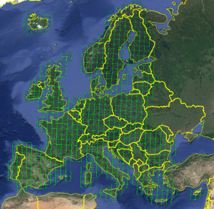
For each tile there are two Geotiff files containing the vertical mean velocity and the east-west mean velocity. Associated with each Geotiff there is a .zip archive file, containing the previously specified CSV file (fields listed in Table 6 from top to bottom are stored as columns from left to right), and XML header file, (with the fields in Table 9). The name of the .zip archive follows the aforementioned convention, and it resembles the name of the contained CSV and XML files, apart from the .zip extension.

6.4 GNSS model product format

The GNSS model is delivered as a single CSV file, with an accompanying XML header file with metadata from the production.

7 Downloading EGMS Products

Detail on how to access EGMS products via the dedicated Dissemination & Archive System is contained in RD3 document.

8 Quality And Accuracy

The quality of EGMS products is of paramount importance in providing a reliable service, and numerous quality checks are made and then verified throughout the production process. Some of the quality checks are available in the products download unit (e.g., temporal_coherence, rmse, amplitude_dispersion, all the standard deviation fields). For more information on the details of EGMS quality control and assurance, please refer to [RD?].

9 Ancillary Datasets

A number of non-InSAR datasets are used in the production and validation of EGMS products. Table 11 below lists these along with a brief comment as to their purpose.

Table 8 Ancillary datasets used in EGMS production
ITEM	COMMENT
Sentinel-1 precise orbit data	Precise orbit information is essential for high-quality InSAR analysis. Precise orbit data are distributed by ESA, with a current latency of about three weeks. See: https://scihub.copernicus.eu/gnss/#/home
Digital Elevation Model	A DEM is needed to compensate for phase changes caused by topographic relief. For EGMS production, the Copernicus DEM GLO-30 (30 m resolution) is used, see: https://spacedata.copernicus.eu/web/cscda/dataset-details?articleId=394198
Land cover data	Landcover influences MP density, and so a common landcover database is used to verify appropriate MP density and ensure consistency. For EGMS, the CLC 2018 CORINE land cover maps are used, see: https://land.copernicus.eu/pan-european/corine-land-cover/clc2018
Snow cover data	The Copernicus Snow Cover Extent product may be used to identify SAR data that is unreliable for InSAR analysis due to snow cover. See: https://land.copernicus.eu/global/products/sce
External datum reference	To anchor and make ‘absolute’ Calibrated and Ortho product measurements, a harmonised GNSS framework is needed. The EUREF and EPN-D networks, along with various derived models are used for this action. See: http://www.epncb.oma.be/ https://epnd.sgo-penc.hu/

10 References

Cooksley, G et al (2004) S5: Service Portfolio Specifications. ESA-Terrafirma project dossier.

Davis, B (2020) Precision and accuracy in glacial geology. AntarcticGlaciers.org. Retrieved 29 March 2021 from: http://www.antarcticglaciers.org/glacial-geology/dating-glacial-sediments-2/precision-and-accuracy-glacial-geology/

11 Appendix A

Note in these sections, EGMS products names are abbreviated to their code-references as follows:

EGMS product name	Code reference
Basic	L2a
Calibrated	L2b
Ortho	L3

11.1 XML Header File

Table 9 XML header file
Product	Field	Spec and notes
L2a + L2b + L3	product_level	L2a, L2b, L3
L2a + L2b	burst_id	See section 11.2
L2a + L2b + L3	production_facility	1 = EGEOS, 2 = GAF, 3 = NORCE, 4 = TREA.
L2a + L2b + L3	production_date	Format dd/mm/yyyy.
L2a + L2b + L3	dem	The version of the Copernicus 30m DEM.
L2a + L2b	corine	Present if used. Version.
L2a + L2b	sce	Present if used. Version.
L2b + L3	GNSS version	Version of the model.
L2a	clusters	0 if there is just one cluster in the CSV file. N if there are more than one clusters in the CSV file (where N is the number of identified clusters).
L2a + L2b	image	Identifies the properties of each image used to generate the deliverable. It contains the tags product_id, and orbit_type.
L2a + L2b	product_id	The actual product name used, stripped of the checksum and of the file type “.SAFE”
L2a + L2b	orbit_type	Relative orbit type used for each image in the processing. It may assume values in the set (AUX_PROQUA, AUX_RESORB, AUX_GNSSRD, AUX_POEORB).
L2a + L2b	reference	Reference image used to generate the deliverable. It contains tag images and the relative sub-tags.
L2a + L2b	dataset	All images used to generate the deliverables (included the reference image). It contains a set of tags image and the relative sub-tags

<?xml version="1.0"?> 
<BURST> 
  <product_level>L2b</product_level> 
  <burst_id>0282</burst_id> 
  <production_facility>2</production_facility> 
  <production_date>02/07/2021</production_date> 
  <dem> 
    <version>EU-DEM v1.1</version> 
  </dem> 
  <corine> 
    <version>2018, Version 2020_20u1</version> 
  </corine> 
  <sce> 
    <version></version> 
  </sce> 
  <gnss> 
    <version>1.0</version> 
  </gnss> 
  <clusters>2</clusters> 
  <reference> 
    <image>               <product_id>S1B_IW_SLC__1SDV_20200624T051142_20200624T051210_022171_02A142</product_id> 
      <orbit_type> AUX_POEORB</orbit_type> 
    </image> 
  </reference> 
  <dataset> 
    <image> 
<product_id>S1A_IW_SLC__1SDV_20201027T170648_20201027T170715_040789_04D780</product_id> 
      <orbit_type> AUX_POEORB</orbit_type> 
    </image> 
    <image> 
<product_id>S1B_IW_SLC__1SDV_20200624T051142_20200624T051210_022171_02A142</product_id> 
      <orbit_type> AUX_POEORB</orbit_type> 
    </image> 
    <image> 
<product_id>S1B_IW_SLC__1SDV_20210728T051142_20210728T051210_022171_02A142</product_id> 
      <orbit_type> AUX_POEORB</orbit_type> 
    </image> 
  </dataset> 
</BURST>

Table 10 Example of XML header file

11.2 Convention for Burst Data Files Names

Each burst file name follows a precise convention, which is specified and implemented in the following python code.

### This code demonstrates how to calculate unique burst cycle ID for Sentinel-1 

import math 
  
## S1 IW timing parameters (NB! Must be 64-bit precision or higher!) 
TPRE  = 2.298687 
TBEAM = 2.758273 
TORB  = 12*86400/175 

def get_egms_burst_id(r, bc, swath, polarization): 
    return "{:03d}-{:04d}-{:s}-{:s}".format(r, bc, swath, polarization)
    
def get_esa_burst_cycle_id(delta_tb): 
    return math.floor((delta_tb - TPRE)/TBEAM) + 1 
    
def get_egms_burst_cycle_id(r, anx_time): 
    # ESA burst cycle ID of first complete burst cycle in relative orbit "r".     
    # NB! This calculation assumes that (r-1)*TORB is not an exact multiple 
    # of TBEAM, which is true for all 175 S1 relative orbits.     
    id_esa_first = get_esa_burst_cycle_id((r-1)*TORB) + 1  

    # ESA burst cycle ID for "anx_time" seconds into relative orbit "r". 
    # Note that "anx_time" is sensing time of middle of a burst.has to be 
    id_esa = get_esa_burst_cycle_id((r-1)*TORB + anx_time) 

    # EGMS burst ID is decomposed into (relative orbit, burst cycle within orbit). 
    return (r, id_esa - id_esa_first + 1) 
 

if __name__ == "__main__": 
    ## Example: burst covering Mulhouse in the EGMS ORR ascending data. 

    ## Product: S1B_IW_SLC__1SDV_20180902T172257_20180902T172324_012539_01721C_6F69.SAFE 

    ## Annotation XML file in <Product>/annotation/: 
    ## s1b-iw2-slc-vv-20180902t172258-20180902t172323-012539-01721c-005.xml 

    # Relative orbit can be found, e.g., in <product>/manifest.safe. 
    r = 88 

    # The following timing for first line of burst can be found in XML as 
    # <swathTiming/burstList/burst> (item #7) 
    anx_time = 775.1918283259 

    # We need to adjust this to middle of burst for this calculation. 
    # Burst size is found in XML as 
    #   <swathTiming/linesPerBurst> 
    az_size = 1508 

    # Azimuth sampling interval is found in XML as 
    #   <imageAnnotation/imageInformation/azimuthTimeInterval> 
    dt_az = 0.0020555563 

    # Adjust timing reference to middle of burst, where 
    # zero doppler time is almost equal to sensing time. 
    # Note: it is sufficient that this calculation is accurate to within 
    # about 0.1 sec, so any line near middle of burst is fine. 
    anx_mid = anx_time + az_size/2*dt_az 
 

    # ESA burst ID calculation 
    #   Should be equal to the following field, that will be present 
    #   in S1 IW SLC products from IPF v3.40. 
    #     <swathTiming/burstList/burst/burstID> 
    bc_id_esa = get_esa_burst_cycle_id((r-1)*TORB + anx_mid) 
    assert bc_id_esa == 187151 

    # EGMS burst cycle ID 
    bc_id_egms = get_egms_burst_cycle_id(r, anx_mid) 
    assert bc_id_egms == (88, 282) 

    # EGMS unique burst ID 
    uid_egms = get_egms_burst_id(*bc_id_egms, "IW2", "VV") 
    assert uid_egms == "088-0282-IW2-VV"

Table 11 Unique burst cycle ID for Sentinel-1

EGMS is a one-delivery-per-year project, and, for each delivery, data is contained in a pre-defined temporal range.

The rule to be applied from the second update inward is a 5 full years nominal time range (e.g., images from 01/01/2018 to 31/12/2022 for the second update, images from 01/01/2019 to 31/12/2023 for the third update, and so on).

The suffix _xxxx_yyyy_z is not applied to deliverables belonging to the Baseline or to the First update.

From the second update inward the suffix _xxxx_yyyy_z is appended immediately before the file extension of the names of all EGMS geographical deliverables (L2a, L2b, and L3 data), where

xxxx is the first nominal year of the 5 full years’ time range in which data are included.
yyyy is the last nominal year of the 5 full years’ time range in which data are included.
z is the version of the delivered data; in case several deliveries of some deliverables are necessary in the same update (e.g., issue fixing). It starts from 1 and is increased by one at each new delivery of the same deliverable belonging to the same update.

The convention will apply to the naming of the zip archives containing the bursts/tiles and to all the contained files (XML, CSV, TIFF).

Some clarifications

xxxx and yyyy are the first and last nominal years of one EGMS update and will be used in the suffix of all the deliverables belonging to that update, no matter the effective period inside the 5 nominal years in which data are available. This means that even if data for a given burst are available just in a subset of the 5 years range (e.g., nominal years from 2018 to 2022, years in which data are available from 2019 to 2021), still the deliverables for that burst will be named after the nominal years (2018 and 2022).
It may happen that one or more deliverables are not uploaded on the platform/archive at the moment in which one update of the service is released to the public. In case a deliverable is added after the release to the public of the service, it will be added with the version number (z) starting from 1.
The suffix added to the file names won’t take part in the generation of the PID for the measurement points contained in the file itself.
Data which will substitute corrupted/wrong one in the EGMS system will have a name following the convention, even if the substituted data won’t be maintained in the archive.

Some examples

Second update (data between 1st January 2018 and 31st December 2022)

EGMS_L2a_088_0282_IW2_VV_2018_2022_1.zip

EGMS_L2b_088_0282_IW2_VV_2018_2022_1.zip

EGMS_L3_E40N28_100km_E_2018_2022_1.zip

Second update (a burst with acquisitions just between 8th July 2018 and 29th October 2021)

EGMS_L2a_076_0391_IW1_VV_2018_2022_1.zip

A correction to the burst belonging to the second update (in case an error is spot in the data)

EGMS_L2a_088_0282_IW2_VV_2018_2022_2.zip

11.3 Measurement Points Codes

Each Basic and Calibrated products measurement point’s code follows a precise convention, which is specified and implemented in the following snipper of code. The MP’s codes are univocal over the entire Europe.

# DP representation of Sentinel-1 IW swath mnemonics 
SWATH = {"IW1": 1, "IW2": 2, "IW3": 3} 
LUT_SWATH = {} 
for key in SWATH: 
    LUT_SWATH[SWATH[key]] = key 

# DP representation of IPE names 
IPE = {"UNDEF": 0, "EGEOS": 1, "GAF": 2, "NORCE": 3, "TREA": 4} 
LUT_IPE = {} 
for key in IPE: 
    LUT_IPE[IPE[key]] = key 

# DP representation of polarization (ordered alphabetically). 
POL = {"HH": 0, "HV": 1,  "VH": 2, "VV": 3} 
LUT_POL = {} 
for key in POL: 
    LUT_POL[POL[key]] = key 

# base62 alphabet 
BASE62="0123456789ABCDEFGHIJKLMNOPQRSTUVWXYZabcdefghijklmnopqrstuvwxyz" 
# base62 to DP lookup table for decoding 
LUT_BASE62 = {} 
for (i, c) in enumerate(BASE62): 
    LUT_BASE62[c] = i 


def encode(n, p, pad=None): 
    if n < 0: 
        raise ValueError("Cannot encode negative numbers.") 
    res = "" 
    while True: 
        n, r = divmod(n, p) 
        res = BASE62[r] + res 
        if n == 0: 
            break 
    if pad is None: 
        return res 
    return res.rjust(pad, BASE62[0]) 


def decode(code, p): 
    n = 0 
    for (i, c) in enumerate(code[::-1]): 
        n += LUT_BASE62[c]* p**i 
    return n 
 

def get_point_id(line, pixel, base, pad=None): 
    # Pixel: 16 bits (0-65535), S1 IW max = about 24,500 
    n = pixel 
    b = 16 
    # Line: 11 bits (0-2047), S1 IW max = about 1,470 
    n += line*(1 << b) 
    b += 11 
    return encode(n, base, pad) 

 
def get_burst_id(track, burstno, swath, pol, base, pad=None): 

    # Polarization: 2 bits (0-3), HH/HV/VH/VV 
    n = POL[pol] 
    b = 2 
    # Swath: 2 bits (1-3), S1: IW1/IW2/IW3 
    n += SWATH[swath]*(1 << b) 
    b += 2 
    # Burst number: 12 bits ( 1-2148 ), S1 IW: 2147.xx burst cycles / orbit 
    n += burstno*(1 << b) 
    b += 12 
    # Track: 8 bits (1-175), S1: 175 orbits per repeat cycle 
    n += track*(1 << b) 
    b += 8 
    return encode(n, base, pad) 

 
def get_uid_b62(ipe, track, burstno, swath, pol, line, pixel): 
    point_id = get_point_id(line, pixel, 62, pad=5) 
    burst_id = get_burst_id(track, burstno, swath, pol, 62, pad=4) 
    ipe_id = BASE62[IPE[ipe]] 
    uid = ipe_id+burst_id+point_id 
    return uid 


def analyze_uid_b62(uid): 
    res = {} 
    res["IPE"] = LUT_IPE[decode(uid[0], 62)] 

    n, i = divmod(decode(uid[1:5],62), 2**2) 
    res["POL"] = LUT_POL[i] 
    n, i = divmod(n, 2**2)     
    res["SWATH"] = LUT_SWATH[i]     
    n, i = divmod(n, 2**12) 
    res["BURSTNO"] = i 
    res["TRACK"]   = n 

    n, i = divmod(decode(uid[5:], 62), 2**16) 
    res["LINE"] = n 
    res["PIXEL"] = i 
    return res 

if __name__ == "__main__": 

    ## Example: 

    ipe = "NORCE" 

    # Components of the burst ID 
    track = 88 
    burstno = 282 
    swath = "IW2" 
    pol = "VV" 

    # Position of pixel within burst, where (0,0) is the 
    # first _valid_ line/pixel for the given burst in the reference scene for coregistration. 
    # * Note 1: If subpixel position estimation is used,  
    # please round to the integer      line/pixel containing      the  
    # measurement point 
    # * Note 2: for multilooked DS measurements, please pick one     
    # line/pixel near the      centre of the multilooked DS, using an  
    #  algorithm that will not change over time. 
    # E.g., simply line = round(mean(lines)), and pixel = round(mean(lines)). This assumes that 
    # There is no full resolution PS in that pixel already, which should be a good assumption (?) 
    line = 1234 
    pixel = 12345 

    ## Point ID - Maximum value for S1 IW: 
    # get_point_id(1470, 24400, 62) = '6WKEy' 
    # -> fits in 5 base62 digits 

    ## Burst ID - Maximum value used for S1 IW: 
    # get_burst_id(175, 2148, "IW3", "VV", 62) = 'mGV1' 
    # -> fits in 4 base62 digits 

    # Calculate the unique point ID to be used for EGMS L2a/L2b products 
    uid_egms = get_uid_b62(ipe, track, burstno, swath, pol, line, pixel) 

    # Calculate the individual parts 
    point_id = get_point_id(line, pixel, 62, pad=5) 
    burst_id = get_burst_id(track, burstno, swath, pol, 62, pad=4) 
    ipe_id = BASE62[IPE[ipe]] 

    # Consistency checks 
    assert uid_egms == ipe_id + burst_id + point_id 
    assert uid_egms == "3ODTn5TNYv" 

    uid_decoded = analyze_uid_b62(uid_egms) 

    print("input:") 
    print("------") 
    print("IPE     : "+ipe) 
    print("POL     : "+pol) 
    print("SWATH   : "+swath) 
    print("BURSTNO : "+str(burstno)) 
    print("TRACK   : "+str(track)) 
    print("LINE    : "+str(line)) 
    print("PIXEL   : "+str(pixel)) 
    print("") 
    print("output") 
    print("------") 
    print("ipe_id   : "+ipe_id) 
    print("burst id : "+burst_id) 
    print("point id : "+point_id) 
    print("uid      : "+uid_egms) 
    print("") 
    print("decoded output") 
    print("------") 
    print(uid_decoded) 

    ## Check whether we got back the input: 
    assert uid_decoded["IPE"] == ipe 
    assert uid_decoded["POL"] == pol 
    assert uid_decoded["SWATH"] == swath 
    assert uid_decoded["BURSTNO"] == burstno 
    assert uid_decoded["TRACK"] == track 
    assert uid_decoded["LINE"] == line 
    assert uid_decoded["PIXEL"] == pixel

Table 12 Unique MP's code over the entire Europe for Basic and Calibrated products.

Each Ortho product measurement point’s code follows a precise convention, outlined by the formula in Table 13.

CODE = base62(IPE) + base62(y/100 * 2^32 + x/100)

Table 13 Unique MP's code over the entire Europe for Ortho products.

11.4 Data Field Evaluation

The evaluation of the fields in Table 5 and Table 6 follows a specific convention which is described and implemented by the following snippet of code.

% File to be used as a "pseudo-code" just to define how the different 
% parameters of EGMS deliverables (L2a) should be computed 
%%%%%%%%%%%%%%%%%%%%%%%%%%%%%%%%%%%%%%%%%%%%%%%%%%%%%%%%%%%%%%%%%%%%%%%%%%%%%% 

% NI is the Number of Images(data) 
% "time" is a column vector with "NI" acquisition dates - starting from 0 - [year] 

%% FORWARD - Generate a Time Series - vector [NI x 1] 
%%%%%%%%%%%%%%%%%%%%%%%%%%%%%%%%%%%%%%%%%%%%%%%%%%%%%%%%%%%%%%%%%%%%%%%%%%%%%% 

NI=300;  %% Number of images 
time=(0:6:(NI-1)*6)'/365; %% [year] 
Velocity     = 5*randn % [mm/yr] 
Acceleration = 2*randn % [mm/yr^2] 
SeasonAmp    = 10*rand % [mm] 
Offset       = rand    % [year] 
noise        = 4*randn(NI,1);     % [mm] 
TimeSeries = 0.5*Acceleration*time.^2 + Velocity*time +... 
    SeasonAmp*cos(2*pi*(time-Offset))+noise; 

%%%%%%%%%%%%%%%%%%%%%%%%%%%%%%%%%%%%%%%%%%%%%%%%%%%%%%%%%%%%%%%%%%%%%%%%%%%%%% 

%%%% TASK 1 - Computation of the RMSE of each Time Series 
%%%%          and estimation of the Amplitude of the Seasonal Component 
%%%%%%%%%%%%%%%%%%%%%%%%%%%%%%%%%%%%%%%%%%%%%%%%%%%%%%%%%%%%%%%%%%%%%%%%%%%%%% 

%%% Model Matrix - Third order polynomial + seasonality  
%%%%%%%%%%%%%%%%%%%%%%%%%%%%%%%%%%%%%%%%%%%%%%%%%%%%%%%%%%%%%%%%%%%%%%%%%%%%% 

G = [time.^3 time.^2 time ones(NI,1) cos(2*pi*time) sin(2*pi*time)]; 

%% inversion 
invG=inv(G'*G);  %% pseudoinverse(Moore-Penrose) 
COEFF = invG*G'*TimeSeries; 
Model=G*COEFF; 

% Compute RMSE 
RMSE = sqrt( mean( (TimeSeries-Model).^2 ) ) %%% [mm] 

% Compute the amplitude of the seasonal component and its StDev 
EstimatedSeasonAMP= sqrt( COEFF(5).^2+COEFF(6).^2 ); 
EstimatedSTD_SeasonAMP= sqrt( (4-pi)/2*(invG(5,5)+invG(6,6))/2 )*RMSE;  
% In fact, this is the StDev of a Rayleigh distribution, since the amp of 
% the seasonal component is sqrt( COEFF(5).^2+COEFF(6).^2 ); and we 
% suppose a gaussian statistics 

Estimated_AMP_And_Std = [EstimatedSeasonAMP EstimatedSTD_SeasonAMP] 

% PLOT THE TIME SERIES 
plot(time,[TimeSeries Model]); 
legend('Data','Model'); 
xlabel('Time [year]'); 
ylabel('Displacement [mm]'); 
grid on 

%%%%%%%%%%%%%%%%%%%%%%%%%%%%%%%%%%%%%%%%%%%%%%%%%%%%%%%%%%%%%%%%%%%%%%%%%%%%%% 

%%%% TASK 2 - Compute Mean Velocity and its StdDev 
%%%%%%%%%%%%%%%%%%%%%%%%%%%%%%%%%%%%%%%%%%%%%%%%%%%%%%%%%%%%%%%%%%%%%%%%%%%%%% 

%%% Model Matrix - First order polynomial + seasonality  
%%%%%%%%%%%%%%%%%%%%%%%%%%%%%%%%%%%%%%%%%%%%%%%%%%%%%%%%%%%%%%%%%%%%%%%%%%%%%% 

G = [time ones(NI,1) cos(2*pi*time) sin(2*pi*time)]; 

%%%%% inversion %%%%%% 
invG=inv(G'*G); 
COEFF = invG*G'*TimeSeries; 
Model=G*COEFF; 
EstimatedVelocity = COEFF(1); %%% [mm/yr] 
EstimatedSTD_Noise = std(TimeSeries-Model); 
EstimatedSTD_Vel = sqrt(invG(1,1))*EstimatedSTD_Noise; %%% in [mm/yr] 
Estimated_Vel_And_Std = [EstimatedVelocity EstimatedSTD_Vel] 


%%%%%%%%%%%%%%%%%%%%%%%%%%%%%%%%%%%%%%%%%%%%%%%%%%%%%%%%%%%%%%%%%%%%%%%%%%%%%% 
%%%% TASK 3 - Compute Acceleration and its StdDev 
%%%%%%%%%%%%%%%%%%%%%%%%%%%%%%%%%%%%%%%%%%%%%%%%%%%%%%%%%%%%%%%%%%%%%%%%%%%%%% 

%%% Model Matrix - Second order polynomial + seasonality  
%%%%%%%%%%%%%%%%%%%%%%%%%%%%%%%%%%%%%%%%%%%%%%%%%%%%%%%%%%%%%%%%%%%%%%%%%%%%%% 

G = [0.5*time.^2 time ones(NI,1) cos(2*pi*time) sin(2*pi*time)];

%%%%% inversion %%%%%% 
invG=inv(G'*G); 
COEFF = invG*G'*TimeSeries; 
Model=G*COEFF; 
EstimatedAcceleration = COEFF(1); %%% [mm/yr] 
EstimatedSTD_Noise = std(TimeSeries-Model); 
EstimatedSTD_Acc = sqrt(invG(1,1))*EstimatedSTD_Noise; %%% in [mm/yr] 
Estimated_Acc_And_Std = [EstimatedAcceleration EstimatedSTD_Acc]

Table 14 Data delivery field evaluation

12 Document Control Information

Settings	Value
Document Title:	Product Description and Format Specification
Project Title:	EGMS-SC1
Project Owner:	Henrik Steen Andersen (EEA)
Document Code:	EGMS-D6-PDD-SC1-2.0-009
Document Version:	2.0
Distribution:	Public
Date:	25/10/2023

Document Approver(s) and Reviewer(s):

Name	Role	Action	Date
Lorenzo Solari	Project Officer (EEA)	Approve	25/10/2023

Document history:

Revision	Date	Short Description of Changes
draft 1.0	18/06/2021	Initial version
draft 1.1	15/10/2021	Updated according to review by EEA
draft 1.2	20/12/2021	Updated according to review by EEA
1.0	24/02/2022	Changes to EGMS Basic data format
2.0	25/10/2023	Changes to EGMS Basic data naming convention

Reuse

EUPL (>= 1.2)

ID	Reference or Related Document	Date	ID	Source or Link/Location
	ALG Algorithm Theoretical Basis	20/12/2021	EGMS-D3-ALG-SC1-2.0-006	EGMS Original Consortium
	Product User Manual	14/02/2022	EGMS-D4-PUM-SC1-2.0-007	EGMS Original Consortium
	End User Interface Manual	15/10/2021	EGMS-D5-UIM-SC1-2.0-008	EGMS Original Consortium
	Product Archive and Dissemination System Description	20/12/2021	EGMS-D9-DAS-SC1-2.0-011	EGMS Original Consortium
	Quality assurance and control report	22/10/2021	EGMS-D10.1-QCR-SC1-3.0-012	EGMS Original Consortium
	User Uptake Plan	15/10/2021	EGMS-D14-UUP-SC1-8.0-016	EGMS Original Consortium
	End User Requirements	20/12/2021	EGMS-D15-URD-SC1-8.0-017	EGMS Original Consortium
	GNSS calibration report	20/12/2021	EGMS-D19.1-GCR-SC1-3.0-014	EGMS Original Consortium